Many natural resource management questions involve a variety of data that are challenging to work with using typical computer resources. The USGS Geo Data Portal (GDP) removes the barrier to these large or complex data by moving processing to the web. This gives researchers and managers access to powerful computers and software tools with minimal effort, enabling them to produce important results with less investment.
The GDP moves computationally intensive processing steps from a researcher's computer to the web. Rather than moving the data to the processing power, the GDP moves the processing power to the data. This means researchers have more computational power available to them and do not need to use their personal computers for lengthy downloads and tedious processing tasks.
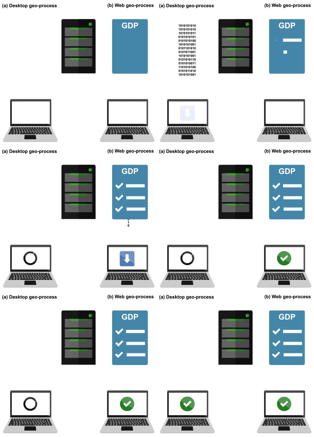
This differs from traditional geoprocessing workflows which often require users to download massive, often terabyte-scale datasets to subset and process. The GDP allows users to download only the subset of the data they need. The average GDP processing job reduces data sent to the user by approximately 90%.
There are a number of built-in algorithms that take the gridded data and distill it. A commonly-used algorithm is area-weighted spatial averages. The GDP will take the gridded dataset and average the data within the given spatial extent. If the dataset has multiple time steps, the GDP will compute a per-feature average for each. The final processed data will be a time series with a value for each time step and each spatial feature.
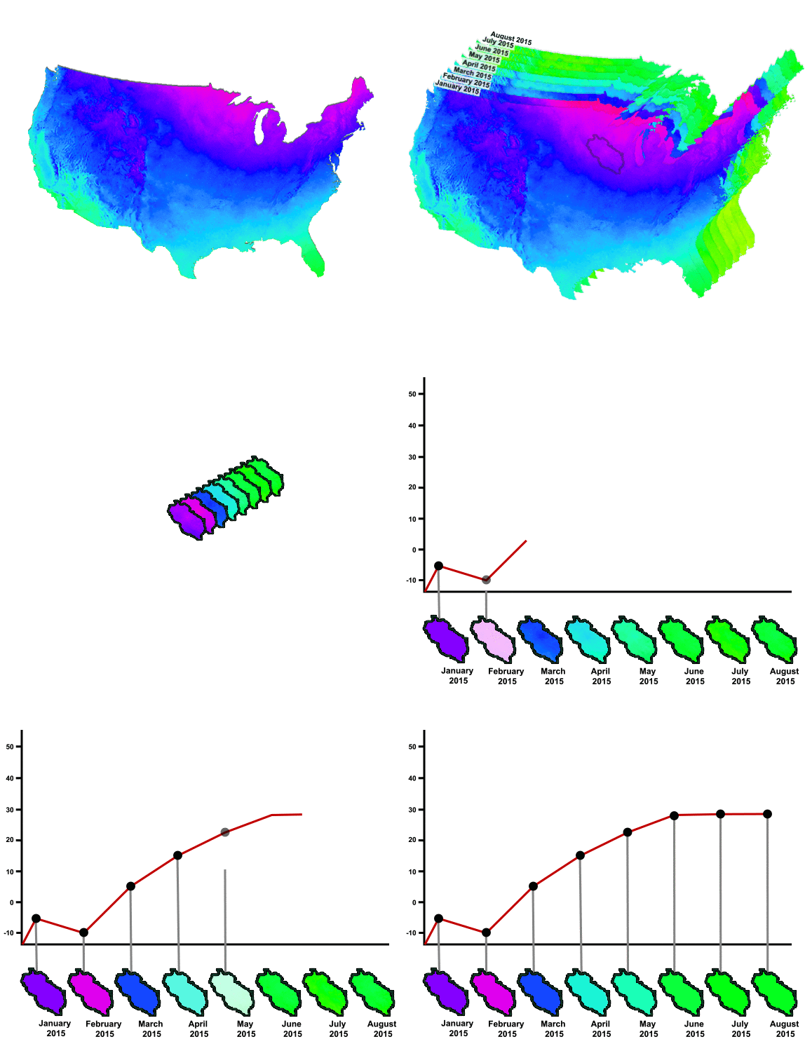
In the figure above, a user is requesting monthly temperature data from January to August 2015 for a feature around Minnesota and Wisconsin. For each month in the temperature dataset, there is a grid of data which is clipped to the spatial feature. Each clipped grid is averaged, leaving one value for each month.
We are using an extreme storm transposition analysis to show the GDP in action. Storm transpositions are a “what-if” water resource planning tool where observations of actual extreme rain events are transposed to different geographic locations. Water resource managers can use this method to evaluate the impact a storm with similar intensity would have on their city and then implement risk-reducing measures where they are needed. In this case, we follow an example from Hayden et al. (2016) where a 2008 extreme storm in Baraboo, WI is transposed to assess the response of the Yahara River watershed (near Madison, WI) to the same kind of weather event. For this example, we are only going to find the cumulative precipitation, and not continue the analysis by using that value for flood modeling.
Here is a visualization product showing the resulting cumulative precipitation from transposing the extreme storm from Baraboo to the Yahara River watershed.
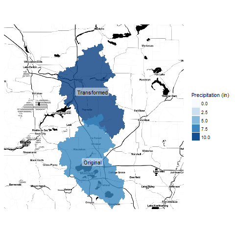
The cumulative precipitation for both the original Yahara (7.6 in) and the transposed Yahara (10.4 in) were calculated, and are shown on the figure above. Transposing the storm north 24 miles resulted in an increase of almost 3 inches of rain. The storm dates were selected from June 2, 2008 to June 13, 2008. A shapefile of the Yahara River watershed was downloaded using the National Water Census Data Portal. To “transpose” the storm, the Yahara shapefile was first shifted north to the center of the extreme storm. This new spatial feature was used as input to the GDP, along with the storm start and end dates, and the area-weighted average algorithm was used to process this data. A dataset of average precipitation for each time step was returned, and the cumulative sum calculated. The cumulative precipitation can now be used as input to flood models and other management tools to determine how this extreme storm could have impacted the Yahara (not covered here). The following will break down how the GDP processed this data.
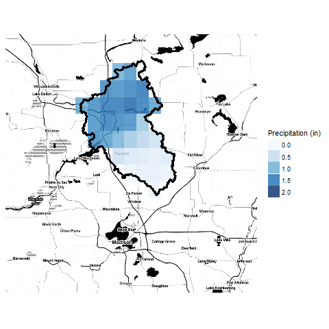
For this analysis, we used precipitation data available in the “United States Stage IV Quantitative Precipitation Archive” dataset from the GDP. The data are gridded and have multiple time steps. Below is an example of the gridded dataset before GDP processing. For simplicity, we are showing a single time step (10:00 pm (UTC) on June 12, 2008).
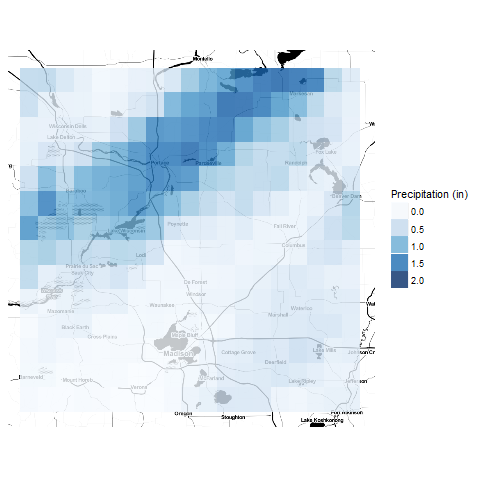
The GDP summarizes the gridded data based on given geometries and algorithms. We transposed the Yahara River watershed north to where the most intense part of the 2008 storm occurred. Using this as our spatial feature means that the GDP will be clipping the gridded dataset with the extreme storm data captured in our Yahara-shaped feature.
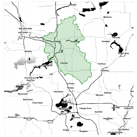
The real power of the GDP is summarizing all of this data. For each time step, the GDP clips the data to the given geometry, and then “melts” the data for that geometry into one value based on your chosen algorithm. The result is one value per time step per geometry, so in this example, one value per time step in the transposed Yahara watershed.
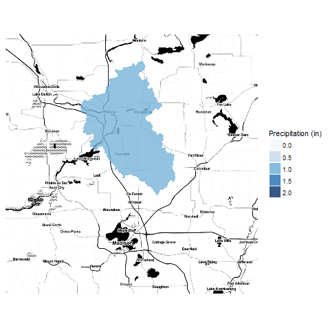
Transposing the Yahara watershed north by 24 miles to capture the highest intensity of the 2008 storm resulted in an increase of 3 inches of rainfall. These precipitation data could now be used in a watershed model, data visualization, or statistical analysis to calculate runoff and streamflow or evaluate the characteristics of the transposed storm. Any of these could also be used to compare the storm that did occur over the Yahara River with the transposed storm.
Results from the GDP can be used for any application that needs input data on a per-feature basis. Environmental modeling applications as well as data summaries and visualizations can use GDP output with little to no additional processing. Examples of analyses that have used the GDP include lake temperature modeling, surface-water modeling, and beach water-quality modeling.